lionheart

Attach sample of the file and the csv output. Also post the code you used to convert the data to csv file to have a look

Change thi line If Target.Value = Empty Then Columns(sColTarget).Rows(FirstRow & ":" & FirstRow + 1).ClearContents: GoTo Skipper To be Columns(sColTarget).Rows(FirstRow & ":" & FirstRow + 1).ClearContents: GoTo Skipper

Try the last point by yourself You can use conditional formatting to do that task

Suppose the cells are B1 & B2 for the year and the month, try the following code in worksheet change event Private Sub Worksheet_Change(ByVal Target As Range) Const FirstRow As Long = 4, FirstColumn As Long = 3, numColumns As Long = 366, sColTarget As String = "C:ND" Dim results(1 To 2, 1 To numColumns), yearValue As Long, currentDate As Date, lastDate As Date, i As Long, selectedMonth As Long, col As Long If Target.Address = "$B$1" Then If Target.Value = Empty Then Columns(sColTarget).Rows(FirstRow & ":" & FirstRow + 1).ClearContents: GoTo Skipper On Error Resume Next yearValue = CInt(Target.Value) On Error GoTo 0 If IsDate("01/01/" & yearValue) Then currentDate = DateSerial(yearValue, 1, 1) lastDate = DateSerial(yearValue + 1, 1, 1) - 1 i = 0 While currentDate <= lastDate i = i + 1 results(1, i) = Format(currentDate, "ddd") results(2, i) = Format(currentDate, "yyyy-mm-dd") currentDate = currentDate + 1 Wend Application.EnableEvents = False Application.ScreenUpdating = False Range(Cells(FirstRow, FirstColumn), Cells(FirstRow + 1, FirstColumn + i - 1)).Value = results Application.ScreenUpdating = True Application.EnableEvents = True Else MsgBox "Please Enter Valid Year", vbExclamation End If ElseIf Target.Address = "$B$2" Then If Target.Value = Empty Then GoTo Skipper On Error Resume Next selectedMonth = Left(Target.Value, InStr(Target.Value, ".") - 1) On Error GoTo 0 If selectedMonth <> 0 Then Application.EnableEvents = False Application.ScreenUpdating = False Columns(sColTarget).Hidden = True For col = FirstColumn To numColumns + (FirstColumn - 1) If IsDate(Cells(FirstRow + 1, col).Value) Then If Month(Cells(FirstRow + 1, col).Value) = selectedMonth Then Cells(FirstRow + 1, col).EntireColumn.Hidden = False End If Next col Application.ScreenUpdating = True Application.EnableEvents = True End If End If Exit Sub Skipper: Application.EnableEvents = False Columns(sColTarget).Hidden = False Application.EnableEvents = True End Sub

But it is not practical to put the year cell and the month cell in L1 & L2 as these columns will be hidden if you select January I suggest you rebuild the strucutre of the file so as to get the year cell and the month cell away from column C to colum NC

What's the expected result in cells C4 and C5

Insert module and paste the following code Sub Highlight_Names_In_Similar_Groups() Dim groupColors(), ws As Worksheet, sh As Worksheet, colRange As Range, cell As Range, sName As String, lr As Long, i As Long Application.ScreenUpdating = False Set ws = ThisWorkbook.Worksheets(2) Set sh = ThisWorkbook.Worksheets(3) Set colRange = ws.Range("E12:N20") lr = sh.Cells(sh.Rows.Count, 3).End(xlUp).Row groupColors = RandomColors(colRange.Columns.Count, True) sh.Columns("C:F").Interior.Color = xlNone For Each cell In colRange.Cells sName = Trim(cell.Value) If sName <> Empty Then For i = 3 To lr If Trim(sh.Cells(i, 3).Value) = sName And sh.Cells(i, 3).Interior.Color <> xlNone Then sh.Cells(i, 4).Resize(, 3).Interior.Color = groupColors(cell.Column - 4) End If Next i End If Next cell Application.ScreenUpdating = True End Sub Function RandomColors(ByVal numColors As Long, Optional ByVal lightColorsOnly As Boolean = False) Dim isUnique As Boolean, i As Long, j As Long ReDim colors(1 To numColors) For i = 1 To numColors Do If lightColorsOnly Then colors(i) = RGB(Int(Rnd() * 128) + 128, Int(Rnd() * 128) + 128, Int(Rnd() * 128) + 128) Else colors(i) = RGB(Int(Rnd() * 256), Int(Rnd() * 256), Int(Rnd() * 256)) End If isUnique = True For j = 1 To i - 1 If colors(i) = colors(j) Then isUnique = False: Exit For Next j Loop Until isUnique Next i RandomColors = colors End Function Then in worksheet module of the first worksheet add this part at the end of the existing code Next c End If If Target.Address = "$C$2" Then Call Highlight_Names_In_Similar_Groups End Sub

Still no clear logic Please this is the last reply from my side, attach clear file with some of the expected results and put some real names for the teacher column as I don't think your attachment is correct

It seems you didn't get what I meant

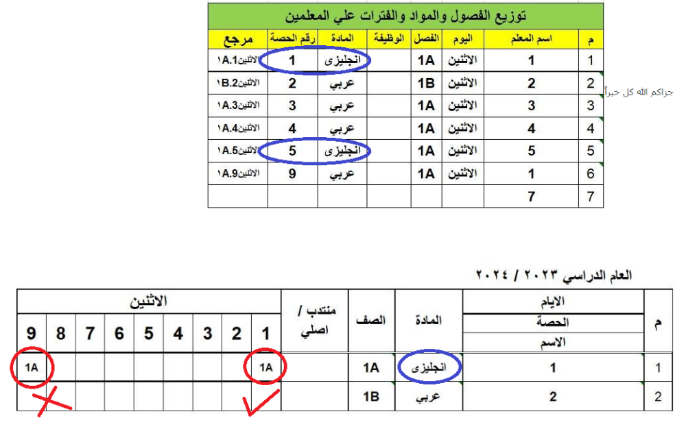
Not logical for me The English subject exists twice for two teachers 1 & 5 so the posted image not correct as for logic English subject should be in the periods 1 & 5 not in 1 & 9

Not clear for me. Please attach sample of the required results

I have no idea about the new request. Please post a new topic with all the required details

Try Sub Test() Dim xDay, xClass, ws As Worksheet, lr As Long, r As Long, xCol As Long Application.ScreenUpdating = False Set ws = ActiveSheet With ws lr = .Cells(Rows.Count, "C").End(xlUp).Row .Range("M7:BE95").ClearContents For r = 7 To lr xDay = Application.Match(.Cells(r, "C").Value, .Rows(5), 0) If Not IsError(xDay) Then xCol = xDay + Val(.Cells(r, "G").Value) - 1 xClass = Application.Match(.Cells(r, "D").Value, .Columns(12), 0) If Not IsError(xClass) Then .Cells(xClass, xCol).Value = .Cells(r, "B").Value .Cells(xClass + 1, xCol).Value = .Cells(r, "F").Value End If End If Next r End With Application.ScreenUpdating = True End Sub

In the code you have this line x = ComboBox1.Value So if you don't select any option from the ComboBox1, you will get the `x` variable equals to empty and this will cause an error You can exit sub by adding this line If x = "" Then MsgBox "Select Option First":Exit Sub

Try the code and if you have any different request please post a new topic Option Explicit Private Sub Worksheet_Change(ByVal Target As Range) Const SROW As Long = 6, EROW As Long = 20, SCOL As Long = 5, ECOL As Long = 8 Dim x, v, rng As Range, cel As Range, c As Long, n As Long If Target.Column = 3 And Target.Row > 15 Then For c = SCOL To ECOL n = 0 If c = 5 Then n = RGB(125, 219, 210) ElseIf c = 6 Then n = RGB(255, 218, 100) ElseIf c = 7 Then n = RGB(155, 200, 95) ElseIf c = 8 Then n = RGB(85, 116, 123) End If With Sheet2 Set rng = .Range(.Cells(SROW, c), .Cells(EROW, c)) x = Application.Match(Target.Offset(, 1).Value, rng, 0) If Not IsError(x) Then For Each cel In rng If Not IsEmpty(cel) Then v = Application.Match(cel.Value, Columns(Target.Offset(, 1).Column), 0) If Not IsError(v) Then Application.EnableEvents = False Cells(v, Target.Column).Value = Target.Value Cells(v, Target.Column).Interior.Color = n Application.EnableEvents = True End If End If Next cel 'Exit For End If End With Next c End If End Sub

Try changing this line and remove Val function v = Application.Match(Val(cel.Value), Columns(Target.Offset(, 1).Column), 0) To be v = Application.Match(cel.Value, Columns(Target.Offset(, 1).Column), 0)

You can use this formula directly =SUM($F$3:F3)>الرئيسي!$D$3

Sub Test() Dim s As String s = Range("C2").Value & Space(1) s = s & Join(Array(Chr(200), Chr(202), Chr(199), Chr(209), Chr(237), Chr(206)), Empty) & Space(1) s = s & Format(Range("C1").Value2, "yyyy/mm/dd") Range("E1").Value = s End Sub

In worksheet module try Private Sub Worksheet_Change(ByVal Target As Range) Const SROW As Long = 6, EROW As Long = 12, SCOL As Long = 3, ECOL As Long = 6 Dim x, v, rng As Range, cel As Range, c As Long If Target.Column = 3 And Target.Row > 15 Then For c = SCOL To ECOL With Sheets(2) Set rng = .Range(.Cells(SROW, c), .Cells(EROW, c)) x = Application.Match(Target.Offset(, 1).Value, rng, 0) If Not IsError(x) Then For Each cel In rng If Not IsEmpty(cel) Then v = Application.Match(Val(cel.Value), Columns(Target.Offset(, 1).Column), 0) If Not IsError(v) Then Application.EnableEvents = False Cells(v, Target.Column).Value = Target.Value Application.EnableEvents = True End If End If Next cel End If End With Next c End If End Sub

Try this Private Sub TextBox1_Change() Dim v() As String v = Split(TextBox1.Value, "-") TextBox2.Value = Format(CDate(v(0)), "dd/mm/yyyy") TextBox3.Value = v(1) End Sub

Sub Test() ProtectWorksheets False Rem YOUR CODE ProtectWorksheets True End Sub Public Sub ProtectWorksheets(ByVal bProtect As Boolean) Const MYPASS As String = "123" Dim ws As Worksheet For Each ws In ThisWorkbook.Worksheets If bProtect = False Then ws.UnProtect Password:=MYPASS Else ws.Protect Password:=MYPASS End If Next ws End Sub

In cell B2 use this formula =DATEVALUE(LEFT(A2,FIND("-",A2)-1)) In cell C2 use this formula =TRIM(RIGHT(A2,LEN(A2)-FIND("-",A2)))

Try Sub Test() Dim x, w, ws As Worksheet, lr As Long Application.ScreenUpdating = False Set ws = ThisWorkbook.Worksheets(1) With ws lr = .Cells(Rows.Count, "B").End(xlUp).Row + 1 x = Application.Match(.Range("D2").Value2, .Rows(6), 0) If Not IsError(x) Then w = Application.Match(.Range("B2").Value, .Range("B7:B" & lr), 0) If Not IsError(w) Then .Cells(w + 6, x).Resize(, .Range("F2").Value).Value = .Range("C2").Value Else .Cells(lr, 1).Value = .Cells(lr, 1).Row - 6 .Cells(lr, 2).Value = .Range("B2").Value .Cells(lr, x).Resize(, .Range("F2").Value).Value = .Range("C2").Value End If End If End With Application.ScreenUpdating = True End Sub

I think this is a different request. Please post a new topic for the new question

Does the code raises any errors? The code is working well on my side. Just select the suitable month as the date in cell D2 is in March and the selected month is February