lionheart

Try Sub Test() Dim ws As Worksheet, sh As Worksheet, tbl As ListObject, lr As Long, i As Long Application.ScreenUpdating = False With ThisWorkbook Set ws = .Worksheets("Items"): Set sh = .Worksheets("Orders") End With Set tbl = sh.ListObjects(1) lr = tbl.Range.Rows.Count + tbl.Range.Row - 1 Do While sh.Cells(lr, "C").Value = Empty lr = lr - 1 Loop lr = lr + 1 Dim a(1 To 16), e For Each e In Split("H15,F4,F6,H6,F9,H9,J9,F13,H13,J13,F15,J15,F18,H18,J18,F20", ",") i = i + 1 a(i) = ws.Range(e).Value Next e sh.Range("C" & lr).Resize(, 16).Value = a Application.ScreenUpdating = True MsgBox "Done", 64 End Sub

Very weird I have commented this line as I didn't want to print Rem sh.PrintOut Rem is used to make the line as a comment. Just remove the Rem and the sheet will be printed Another point I have put this line just for wait, you can remove this line Application.Wait Now + TimeValue("00:00:01") Try to understand the code. Don't wait others to do the whole work for you

Try Sub Test() Dim a, e, ws As Worksheet, sh As Worksheet, i As Long Set ws = ThisWorkbook.Worksheets(1): Set sh = ThisWorkbook.Worksheets(2) a = ws.Range("B11:J" & ws.Cells(Rows.Count, "B").End(xlUp).Row).Value e = sh.Range("Q3").Value For i = LBound(a) To UBound(a) If a(i, 8) = e Then sh.Range("F9").Value = a(i, 2) sh.Range("M9").Value = a(i, 9) Application.Wait Now + TimeValue("00:00:01") Rem sh.PrintOut End If Next i End Sub

Try Sub Test() Dim lr As Long With ActiveSheet lr = .Cells(Rows.Count, 1).End(xlUp).Row With .Sort .SortFields.Clear .SortFields.Add Key:=Range("F3"), Order:=xlAscending .SortFields.Add Key:=Range("G3"), Order:=xlDescending .SortFields.Add Key:=Range("H3"), Order:=xlAscending .SetRange ActiveSheet.Range("A3:H" & lr) .Header = xlYes .Apply End With End With End Sub

Try this code Sub Test() Dim wk As Worksheet, sh As Worksheet, ws As Worksheet, lr As Long Set wk = ThisWorkbook.Worksheets(1) Set sh = ThisWorkbook.Worksheets(2) Set ws = CopyWorksheet(wk.Name, wk.Range("B5").Value) Application.ScreenUpdating = False With sh lr = .Cells(Rows.Count, "J").End(xlUp).Row + 1 .Range("B" & lr).Resize(, 5).Value = wk.Range("B5").Resize(, 5).Value .Range("I" & lr).Resize(, 3).Value = Array(wk.Range("D13").Value, wk.Range("D23").Value, wk.Range("D30").Value) .Range("L" & lr).Formula = "=SUM(I" & lr & ":K" & lr & ")" .Range("N" & lr).Value = wk.Range("F41").Value Application.Goto .Range("A1") End With Application.ScreenUpdating = True End Sub Function CopyWorksheet(ByVal sheetName As String, ByVal newName As String) As Worksheet Application.ScreenUpdating = False On Error Resume Next Application.DisplayAlerts = False ThisWorkbook.Worksheets(newName).Delete Application.DisplayAlerts = True On Error GoTo 0 ThisWorkbook.Worksheets(sheetName).Copy After:=ThisWorkbook.Sheets(ThisWorkbook.Sheets.Count) ActiveSheet.Name = newName Set CopyWorksheet = ActiveSheet Application.ScreenUpdating = True End Function

In worksheet module paste the following code Private Sub Worksheet_Change(ByVal Target As Range) Dim x If Target.Row > 4 And Target.Column = 1 Then x = Application.Match(Target.Value, Sheets(2).Columns(1), 0) If Not IsError(x) Then Target.Offset(, 1).Value = Sheets(2).Cells(x, 2).Value End If End If End Sub

In cell B3 type the formula =COUNTIFS($J$2:$J$100,A3,$Q$2:$Q$100,"*-*")

Insert Module1 and paste the following code Option Explicit Private Sub ColorBySubject() Const STARTROW As Long = 8, STARTCOL As Long = 5, COLSNUM As Long = 4 Dim x, aCols, wsMarks As Worksheet, wsColors As Worksheet, rng As Range, sMarks As String, sQuote As String, sCell As String, n As Long, m As Long, ii As Long Application.ScreenUpdating = False With ThisWorkbook Set wsMarks = .Worksheets(1) Set wsColors = .Worksheets(2) End With Set rng = wsColors.Range("S8:S15") x = Application.Match(wsColors.Range("E3").Value, rng, 0) If Not IsError(x) Then sMarks = wsMarks.Name sQuote = WorksheetFunction.Rept(Chr(34), 2) n = wsMarks.Cells(Rows.Count, "C").End(xlUp).Row - 3 aCols = Array(5, 8, 11, 14, 17, 20, 23, 26) For m = 1 To 3 sCell = ColumnToLetter(aCols(x - 1) + m - 1) & "4" With wsColors If m <> 3 Then For ii = 4 To 1 Step -1 With .Cells(STARTROW, m * COLSNUM - ii + STARTCOL).Resize(n) .Formula = "=IF(" & sMarks & "!" & sCell & "=" & sQuote & "," & sQuote & ",IF(" & sMarks & "!" & sCell & "=" & ii & ",""0""," & sQuote & "))" End With Next ii Else With .Cells(STARTROW, 13).Resize(n) .Formula = "=IF(" & sMarks & "!" & sCell & "=" & sQuote & "," & sQuote & ",IF(" & sMarks & "!" & sCell & ">=3.5,""0""," & sQuote & "))" .Offset(, 1).Formula = "=IF(" & sMarks & "!" & sCell & "=" & sQuote & "," & sQuote & ",IF(AND(" & sMarks & "!" & sCell & ">=2.5," & sMarks & "!" & sCell & "<3.5),""0""," & sQuote & "))" .Offset(, 2).Formula = "=IF(" & sMarks & "!" & sCell & "=" & sQuote & "," & sQuote & ",IF(AND(" & sMarks & "!" & sCell & ">1," & sMarks & "!" & sCell & "<2.5),""0""," & sQuote & "))" .Offset(, 3).Formula = "=IF(" & sMarks & "!" & sCell & "=" & sQuote & "," & sQuote & ",IF(" & sMarks & "!" & sCell & "=1,""0""," & sQuote & "))" End With End If End With Next m End If Application.ScreenUpdating = True End Sub Function ColumnToLetter(ByVal columnNumber As Long) As String If columnNumber < 1 Then Exit Function ColumnToLetter = UCase(ColumnToLetter(Int((columnNumber - 1) / 26)) & Chr(((columnNumber - 1) Mod 26) + Asc("A"))) End Function Then in worksheet module (Colors) [The worksheet that has the data validation list], paste the following code Private Sub Worksheet_Change(ByVal Target As Range) If Target.Cells.CountLarge > 1 Then Exit Sub If Target.Address = "$E$3" Then Application.Run "Module1.ColorBySubject" End If End Sub

Simply you can filter by color then select the colored cells and paste them to the target range

Solution here

Try this code Sub Test() Const NROWS As Long = 10 Dim a, ws As Worksheet, sh As Worksheet, r As Range, s As String, m As Long, i As Long With ThisWorkbook Set ws = .Worksheets(1): Set sh = .Worksheets(2) End With s = Join(Array(Chr(199), Chr(225), Chr(209), Chr(222), Chr(227)), Empty) m = 2 Set r = sh.Columns(2) a = FindNext(s, r) If Not IsEmpty(a) Then For i = LBound(a) To UBound(a) With sh.Range("A" & a(i)).CurrentRegion.Offset(1) .ClearContents: .Borders.Value = 0 End With sh.Range("A" & a(i) + 1).Resize(NROWS).Value = Evaluate("ROW(1:" & NROWS & ")") sh.Range("B" & a(i) + 1).Resize(NROWS).Value = ws.Range("A" & m).Resize(NROWS).Value m = m + NROWS Next i End If End Sub Function FindNext(ByVal strFind As String, ByVal rng As Range) Dim arr(), myRng As Range, iRow As Long, k As Long With rng Set myRng = .Find(What:=strFind, After:=rng.Cells(rng.Cells.Count), LookIn:=xlValues, LookAt:=xlPart) If Not myRng Is Nothing Then iRow = myRng.Row Do k = k + 1 ReDim Preserve arr(1 To k) arr(k) = myRng.Row Set myRng = .FindNext(myRng) Loop Until myRng.Row = iRow End If End With FindNext = arr End Function Note the following The code will find the rows that has the string `NUMBER` then to copy 10 numbers from the first worksheet and so on But the code is limited to the headers in the second worksheet so not all the numbers in the first worksheet will be copied

Learn the basics my bro Just instead of using CurrentRegion feature change the range you are dealing with example Sub Test() Dim lr As Long With ActiveSheet lr = .Cells(Rows.Count, 1).End(xlUp).Row a = .Range("A2:Z" & lr).Value End With End Sub

Add the following line MsgBox .Columns.Count After this line With Sheets("B1DataT1").Cells(1).CurrentRegion You will get the result 17 columns, so the columns numbers you used are not in the range you are dealing with. That's why you got REF error

Select the desired row and right-click to copy Select one cell then go to the Name Box and type A5144 Right-click and paste

You can use UDF in that case Function GetSheetName(ByVal rng As Range) As String Dim sFormula As String, m As Long, n As Long sFormula = rng.Formula m = InStr(sFormula, "!") If m > 0 Then GetSheetName = Trim(Mid(sFormula, 2, m - 2)) Else GetSheetName = Empty End Function

https://techno7asry.com/forum/t6567

Can you attach a sample file to test on

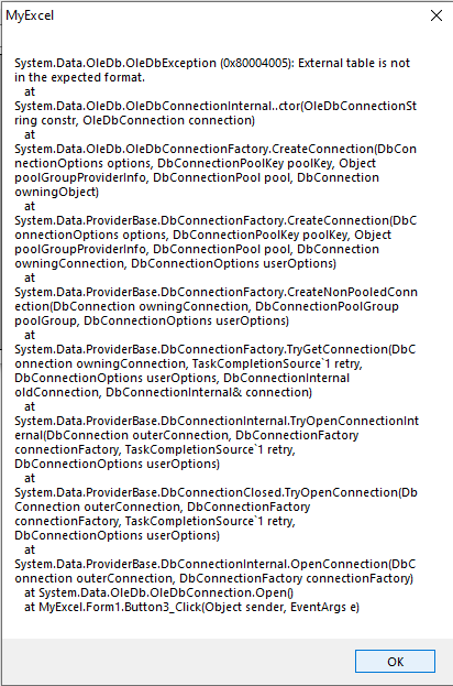
Thank you very much I have encountered an error

Use this macro in the same module Sub Test1() Call CommandButton1_Click Call CommandButton2_Click End Sub If you need to execute the commands away from their module you can use Application.Run Sub Test2() Application.Run "Sheet1.CommandButton1_Click" Application.Run "Sheet1.CommandButton2_Click" End Sub

Ok. No problem at all. I would like to test that software Thanks a lot

There must be trial version. Generally I will continue to follow this topic

Try this code Sub Test() Dim rng As Range, iRow As Long, lr As Long, m As Long Application.ScreenUpdating = False With ActiveSheet .Columns("E:H").ClearContents lr = .Cells(Rows.Count, 1).End(xlUp).Row + 1 m = 3 For iRow = 4 To lr If .Cells(iRow, "B").Value <> .Cells(iRow - 1, "B").Value Then Set rng = .Range("A" & m & ":A" & iRow - 1) .Cells(iRow - 1, "E").Value = .Cells(iRow - 1, "B").Value .Cells(iRow - 1, "F").Value = CountUniqueValues(rng) .Cells(iRow - 1, "G").Formula = "=SUM(" & rng.Offset(, 2).Address(0, 0) & ")" .Cells(iRow - 1, "H").Formula = "=SUM(" & rng.Offset(, 3).Address(0, 0) & ")" m = iRow End If Next iRow End With Application.ScreenUpdating = True MsgBox "Done", 64 End Sub Function CountUniqueValues(ByVal rng As Range) As Long Dim cel As Range, dict As Object Set dict = CreateObject("Scripting.Dictionary") For Each cel In rng If Not dict.Exists(cel.Value) Then dict.Add cel.Value, 1 Next cel CountUniqueValues = dict.Count End Function

Is it free or paid If paid how much

First manually unprotect the worksheet Select column O or just select the cells you would like to deal with Right-Click the selection and select the command Format Cells Go to Protection tab Uncheck the option Locked Protect the worksheet again Please when posting a question, put a suitable title for the topic

Just change to be greater than or equals zero =LOOKUP(2,1/($A$4:$A$23>=0),$B$4:$B$23) Another formula =INDEX($B$4:$B$23,MAX(IF($A$4:$A$23>=0,ROW($A$4:$A$23)-ROW(A4)+1)))